
4. Feature Importances
Contents
4. Feature Importances#
# Loading libraries
from sklearn.model_selection import train_test_split
from sklearn.linear_model import LinearRegression
from sklearn.tree import DecisionTreeRegressor
from sklearn.ensemble import RandomForestRegressor
from sklearn.metrics import mean_squared_error, mean_absolute_error
from sklearn.model_selection import GridSearchCV
from sklearn import tree
# Loading cleaned data
df_features_combined = pd.read_csv('data/df_features_combined.csv')
df_features_combined.shape
(19387, 16)
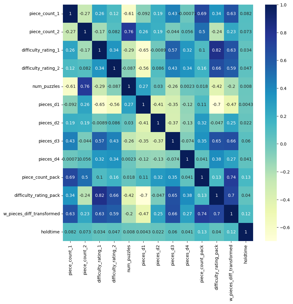
# plotting correlation heatmap
plt.figure(figsize=(10,10))
dataplot = sns.heatmap(df_features_combined.corr(), cmap="YlGnBu", annot=True)

# displaying heatmap
plt.show()
# random split into train and validation
train, test = train_test_split(df_features_combined, test_size = 0.25, random_state=1)
x_train = train.drop(['holdtime', 'pack_name'], axis=1)
y_train = train['holdtime']
x_test = test.drop(['holdtime', 'pack_name'], axis = 1)
y_test = test['holdtime']
4.1 Benchmark Model#
# First just try average hold time by member
train_holdtime_mean = y_train.mean()

pred1 = np.empty(len(y_test))
pred1.fill(train_holdtime_mean)

mean_absolute_error(y_test, pred1)
12.62234436965736
4.2 Linear Regression#
# dummy variable - hopefully x_test doesnt bring any surprises
x_train = pd.get_dummies(x_train)
x_test = pd.get_dummies(x_test)
x_train.shape, x_test.shape
((14540, 32), (4847, 32))
# simple linear regression
model_lr = LinearRegression(normalize=True)
model_lr.fit(x_train, y_train)  #fit the model
pred2 = model_lr.predict(x_test) #make prediction on test set
mean_absolute_error(y_test, pred2) #calculate mae
12.422053647064944
coefficients = pd.concat([pd.DataFrame(x_train.columns,columns=['columns']),
                          pd.DataFrame(np.transpose(model_lr.coef_),columns=['coefficients'])], axis = 1)
coefficients.sort_values(by = 'coefficients').head(15)
| columns | coefficients | |
|---|---|---|
| 0 | piece_count_1 | -5.427657e+11 |
| 1 | piece_count_2 | -5.427657e+11 |
| 29 | brand_2_Stave | -4.353840e+00 |
| 16 | brand_1_Nautilus | -2.782904e+00 |
| 18 | brand_1_Other-Laser-cut | -2.748214e+00 |
| 27 | brand_2_Other-Hand-cut | -1.944098e+00 |
| 13 | brand_1_DaVici | -1.835529e+00 |
| 4 | num_puzzles | -1.622190e+00 |
| 15 | brand_1_Liberty | -1.421600e+00 |
| 20 | brand_1_Wentworth | -1.149477e+00 |
| 22 | brand_2_Artifact | -1.019384e+00 |
| 21 | brand_1_unknown | -9.244420e-01 |
| 2 | difficulty_rating_1 | -2.347115e-01 |
| 3 | difficulty_rating_2 | -1.867834e-01 |
| 17 | brand_1_Other-Hand-cut | 4.988677e-02 |
Cannot say anything about the coefficients right now. Need p-values. Building OLS model to get that.
4.3 OLS model#
from sklearn import datasets, linear_model
import statsmodels.api as sma
X = x_train
y = y_train
X2  = sma.add_constant(X)
est = sma.OLS(y, X2.astype(float))
est2 = est.fit()
print(est2.summary())
                            OLS Regression Results
==============================================================================
Dep. Variable:               holdtime   R-squared:                       0.025
Model:                            OLS   Adj. R-squared:                  0.023
Method:                 Least Squares   F-statistic:                     13.29
Date:                Wed, 15 Mar 2023   Prob (F-statistic):           6.21e-61
Time:                        00:14:09   Log-Likelihood:                -63076.
No. Observations:               14540   AIC:                         1.262e+05
Df Residuals:                   14511   BIC:                         1.264e+05
Df Model:                          28
Covariance Type:            nonrobust
=============================================================================================
                                coef    std err          t      P>|t|      [0.025      0.975]
---------------------------------------------------------------------------------------------
const                        10.5168      2.925      3.596      0.000       4.784      16.250
piece_count_1                 0.0016      0.001      1.216      0.224      -0.001       0.004
piece_count_2                 0.0034      0.002      2.226      0.026       0.000       0.006
difficulty_rating_1          -0.2139      0.532     -0.402      0.688      -1.257       0.829
difficulty_rating_2          -0.2403      0.454     -0.529      0.597      -1.130       0.650
num_puzzles                  -1.5342      0.847     -1.811      0.070      -3.195       0.126
pieces_d1                     0.0014      0.001      1.044      0.297      -0.001       0.004
pieces_d2                    -0.0005      0.001     -0.756      0.449      -0.002       0.001
pieces_d3                    -0.0011      0.001     -1.180      0.238      -0.003       0.001
pieces_d4                     0.0052      0.002      2.568      0.010       0.001       0.009
piece_count_pack              0.0050      0.002      2.839      0.005       0.002       0.008
difficulty_rating_pack        0.3769      0.646      0.583      0.560      -0.890       1.644
w_pieces_diff_transformed     1.3435      0.974      1.379      0.168      -0.566       3.252
brand_1_Artifact              4.5053      0.958      4.705      0.000       2.628       6.382
brand_1_DaVici               -0.0230      2.007     -0.011      0.991      -3.957       3.911
brand_1_Ecru                  2.3095      0.986      2.342      0.019       0.377       4.242
brand_1_Liberty               0.3715      1.121      0.331      0.740      -1.826       2.570
brand_1_Nautilus             -0.9866      1.546     -0.638      0.523      -4.017       2.044
brand_1_Other-Hand-cut        1.8460      1.233      1.497      0.134      -0.571       4.263
brand_1_Other-Laser-cut      -0.8987      1.351     -0.665      0.506      -3.548       1.750
brand_1_Stave                 1.8465      1.407      1.312      0.189      -0.912       4.605
brand_1_Wentworth             0.6735      1.239      0.543      0.587      -1.756       3.103
brand_1_unknown               0.8729      1.526      0.572      0.567      -2.118       3.864
brand_2_Artifact              0.2771      0.901      0.308      0.758      -1.488       2.042
brand_2_DaVici                1.8875      1.955      0.965      0.334      -1.945       5.720
brand_2_Ecru                  1.9655      0.914      2.151      0.032       0.174       3.757
brand_2_Liberty               1.8286      1.128      1.620      0.105      -0.383       4.041
brand_2_Nautilus              3.6361      1.610      2.258      0.024       0.480       6.792
brand_2_Other-Hand-cut       -0.6691      1.178     -0.568      0.570      -2.979       1.641
brand_2_Other-Laser-cut       1.4615      1.260      1.160      0.246      -1.009       3.932
brand_2_Stave                -3.2194      2.467     -1.305      0.192      -8.056       1.617
brand_2_Wentworth             1.5982      1.318      1.213      0.225      -0.985       4.181
brand_2_unknown               1.7507      1.341      1.306      0.192      -0.878       4.379
==============================================================================
Omnibus:                     9068.435   Durbin-Watson:                   1.999
Prob(Omnibus):                  0.000   Jarque-Bera (JB):            97048.061
Skew:                           2.910   Prob(JB):                         0.00
Kurtosis:                      14.239   Cond. No.                     1.14e+16
==============================================================================

Notes:
[1] Standard Errors assume that the covariance matrix of the errors is correctly specified.
[2] The smallest eigenvalue is 9.68e-23. This might indicate that there are
strong multicollinearity problems or that the design matrix is singular.

4.4 Decision Tree#
def dtree_grid_search(X,y,nfolds):
    #create a dictionary of all values we want to test
    param_grid = {'max_depth': [3, 5, 7, 9, 11, 15, 17]}
    # decision tree model
    dtree_model = DecisionTreeRegressor()
    #use gridsearch to test all values
    dtree_gscv = GridSearchCV(dtree_model, param_grid, cv=nfolds)
    #fit model to data
    dtree_gscv.fit(X, y)
    return dtree_gscv.best_params_
dtree_grid_search(X = x_train, y = y_train, nfolds = 5)
{'max_depth': 3}
model_dt = DecisionTreeRegressor(max_depth = 3,random_state=0)
model_dt.fit(x_train, y_train)  #fit the model
pred3 = model_dt.predict(x_test) #make prediction on test set
mean_absolute_error(y_test, pred3) #calculate mae
12.447865314968272
feats = {} # a dict to hold feature_name: feature_importance
for feature, importance in zip(x_train.columns, model_dt.feature_importances_):
    feats[feature] = importance #add the name/value pair

importances = pd.DataFrame.from_dict(feats, orient='index').rename(columns={0: 'Gini-importance'})
# importances.sort_values(by='Gini-importance').plot(kind='bar', rot=45)
importances.sort_values(by = 'Gini-importance', ascending=False).head(15)
| Gini-importance | |
|---|---|
| piece_count_pack | 0.607699 |
| w_pieces_diff_transformed | 0.258662 |
| brand_1_Artifact | 0.088650 |
| pieces_d3 | 0.044989 |
| brand_2_Ecru | 0.000000 |
| brand_1_Wentworth | 0.000000 |
| brand_1_unknown | 0.000000 |
| brand_2_Artifact | 0.000000 |
| brand_2_DaVici | 0.000000 |
| piece_count_1 | 0.000000 |
| brand_1_Other-Laser-cut | 0.000000 |
| brand_2_Liberty | 0.000000 |
| brand_2_Nautilus | 0.000000 |
| brand_2_Other-Hand-cut | 0.000000 |
| brand_2_Other-Laser-cut | 0.000000 |
4.4 Random Forest#
def rf_grid_search(X,y,nfolds):
    param_grid = {'max_depth': [3, 5, 7, 9], 'n_estimators': [50, 70, 100, 150, 200]}
    rf_model = RandomForestRegressor()
    rf_gscv = GridSearchCV(rf_model, param_grid, cv=nfolds)
    rf_gscv.fit(X, y)
    return rf_gscv.best_params_
rf_grid_search(X = x_train, y = y_train, nfolds = 5)
{'max_depth': 3, 'n_estimators': 100}
model_rf = RandomForestRegressor(max_depth = 3,n_estimators=200, random_state=0)
model_rf.fit(x_train, y_train)  #fit the model
pred4 = model_rf.predict(x_test) #make prediction on test set
mean_absolute_error(y_test, pred4) #calculate mae
12.436204414656602
feats_rf = {} # a dict to hold feature_name: feature_importance
for feature, importance in zip(x_train.columns, model_rf.feature_importances_):
    feats_rf[feature] = importance #add the name/value pair

importances_rf = pd.DataFrame.from_dict(feats_rf, orient='index').rename(columns={0: 'feature_importance'})
# importances.sort_values(by='Gini-importance').plot(kind='bar', rot=45)
importances_rf.sort_values(by='feature_importance', ascending=False).head(15)
| feature_importance | |
|---|---|
| piece_count_pack | 0.575958 |
| w_pieces_diff_transformed | 0.213131 |
| brand_1_Artifact | 0.046877 |
| piece_count_1 | 0.043080 |
| pieces_d4 | 0.033324 |
| piece_count_2 | 0.016813 |
| pieces_d3 | 0.015915 |
| pieces_d1 | 0.015663 |
| pieces_d2 | 0.011825 |
| difficulty_rating_1 | 0.007307 |
| brand_2_Ecru | 0.004491 |
| difficulty_rating_pack | 0.003580 |
| brand_2_Artifact | 0.002352 |
| brand_1_Stave | 0.001416 |
| brand_2_Other-Laser-cut | 0.001191 |